[ML/DL 1] 경사하강법 (Gradient Descent)

2022-07-24 3 분 소요

Author : Songho Lee
Date
- First Published: July 24, 2022
- Last modified: -

경사하강법 (Gradient Descent)

1. Introduction

Test post가 아닌 첫 포스팅입니다.
조그만 것부터 시작해보겠습니다.

2. Details

본 포스팅은 인공지능이 weight와 bias를 업데이트하는 원리인 Gradient Descent에 관한 것입니다.

2.1 수식

W_gradient = Learning_rate * mean((y_pred-y_label)*x_data)
b_gradient = Learning_rate * mean((y_pred-y_label)*1)

2.2 코드

import numpy as np
import matplotlib.pyplot as plt

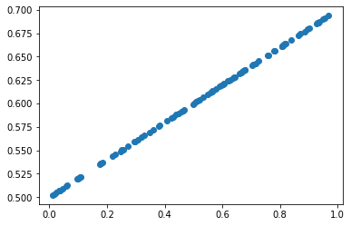
X = np.random.rand(100)
Y = 0.2*X + 0.5

# plt.figure(figsize=(8,6))
plt.scatter(X,Y)
plt.show()

output_7_0

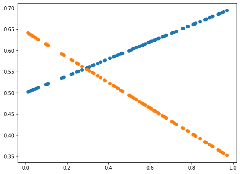
def plot_prediction(pred, y):
  # plt.figure(figsize=(8,6))
  plt.scatter(X, y)
  plt.scatter(X, pred)
  plt.show()

# Gradient Descent 구현
W = np.random.uniform(-1, 1)
b = np.random.uniform(-1, 1)

learning_rate = 0.7

for epoch in range(100):
  Y_Pred = W*X + b

  error = np.abs(Y_Pred - Y).mean()
  if error < 0.001:
    break

  # W, b의 Gradient 계산
  W_grad = learning_rate*((Y_Pred-Y)*X).mean()
  b_grad = learning_rate*((Y_Pred-Y)*1).mean()
  
  # W, b의 갱신
  W = W - W_grad
  b = b - b_grad

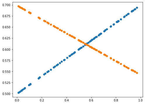
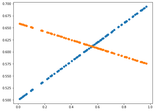
  if epoch % 5 == 0:
    Y_Pred = W*X + b
    plot_prediction(Y_Pred, Y)

output_9_0

output_9_1

output_9_2

output_9_3

output_9_4

output_9_5

output_9_6

output_9_7

output_9_8

output_9_9

output_9_10

output_9_11

output_9_12

output_9_13

output_9_14

output_9_15

output_9_16

output_9_17

output_9_18

output_9_19

print(error)

0.0014589678181387666

2.3 활용

import numpy as np
import matplotlib.pyplot as plt

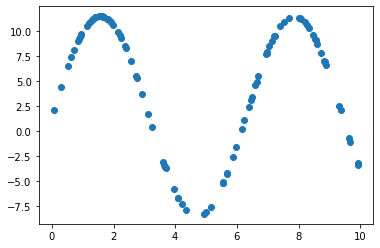
X = np.random.rand(100) * 10
Y = 10 * np.sin(X) + 1.5

plt.scatter(X,Y)
plt.show()

output_13_0

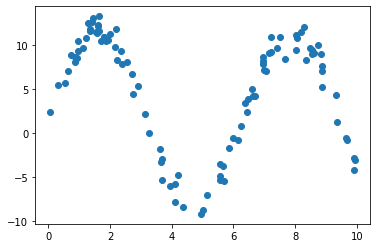
# 노이즈가 있는 데이터에서도 원래의 모델 파라미터를 잘 예측할까?
noise = np.random.normal(0,1,100)

Y_1 = 10 * np.sin(X) + 1.5 + noise

plt.scatter(X,Y_1)
plt.show()

output_14_0

def plot_prediction(pred, y):
  # plt.figure(figsize=(8,6))
  plt.scatter(X, y)
  plt.scatter(X, pred)
  plt.show()

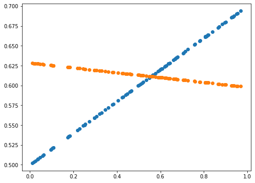
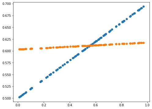
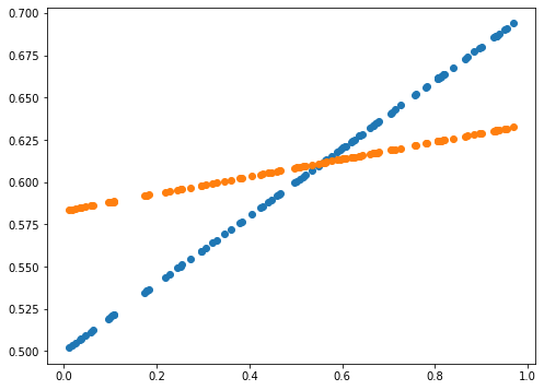
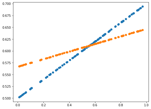
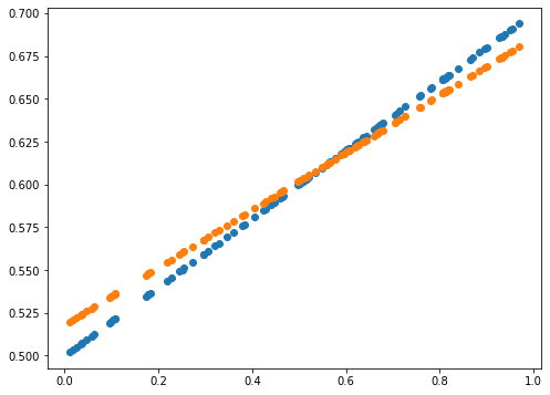
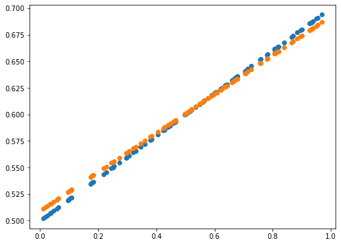
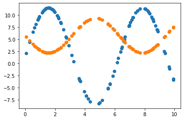
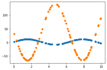
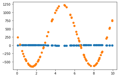
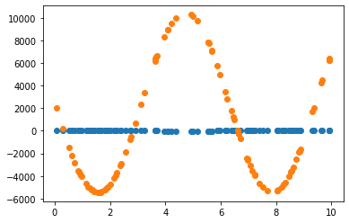
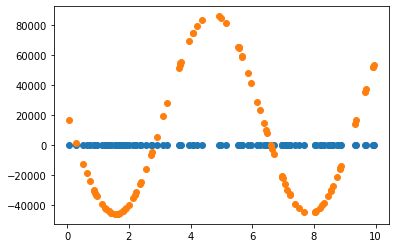
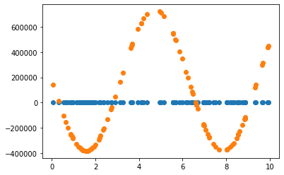
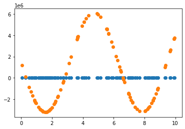
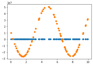
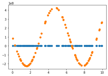
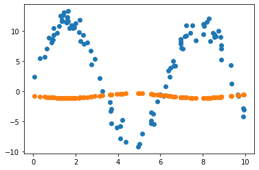
2.3.1 Learning rate = 0.7 그대로 사용

# Gradient Descent 구현 1
W = np.random.uniform(-1, 1)
b = np.random.uniform(-1, 1)

learning_rate = 0.7

for epoch in range(200):
  Y_Pred = W * np.sin(X) + b

  error = np.abs(Y_Pred - Y).mean()
  if error < 0.001:
    break

  # W, b의 Gradient 계산
  W_grad = learning_rate*((Y_Pred-Y)*X).mean()
  b_grad = learning_rate*((Y_Pred-Y)*1).mean()
  
  # W, b의 갱신
  W = W - W_grad
  b = b - b_grad

  if epoch % 20 == 0:
    Y_Pred = W * np.sin(X) + b
    plot_prediction(Y_Pred, Y)

output_17_0

output_17_1

output_17_2

output_17_3

output_17_4

output_17_5

output_17_6

output_17_7

output_17_8

output_17_9

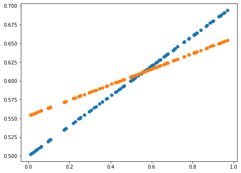
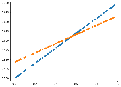
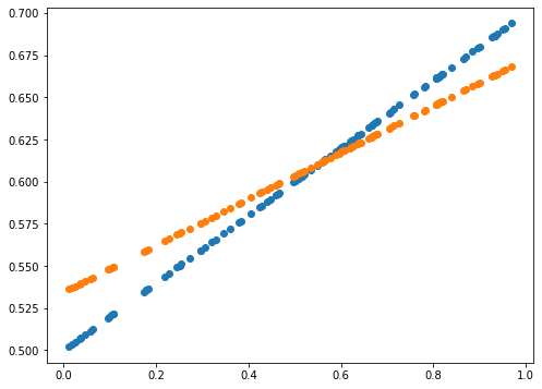
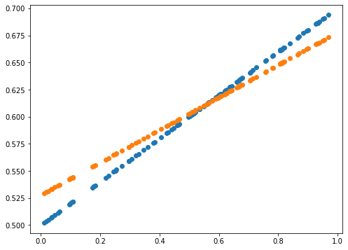
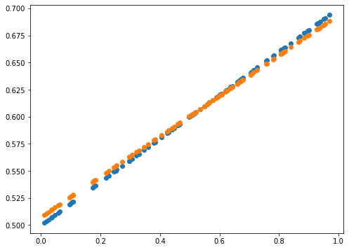
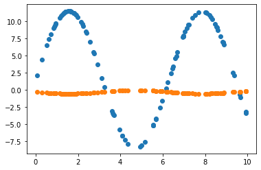
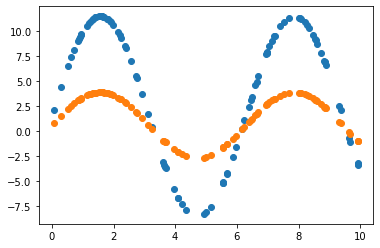
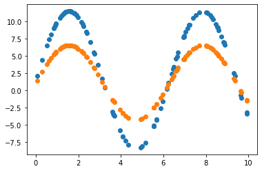
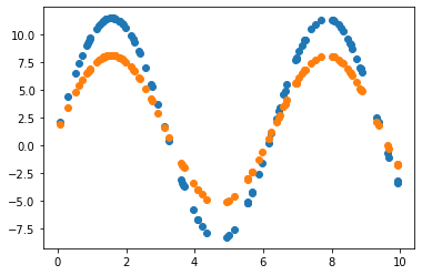
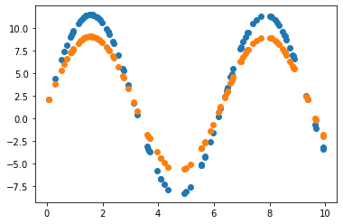
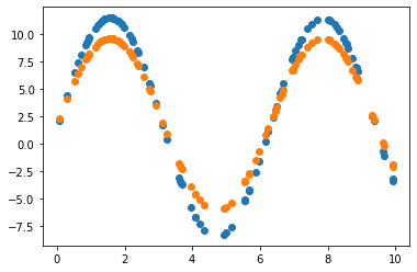
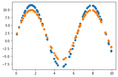
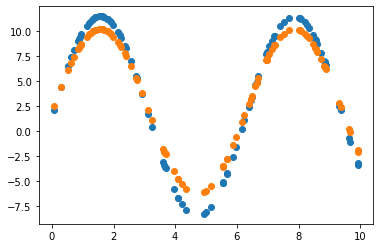
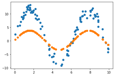
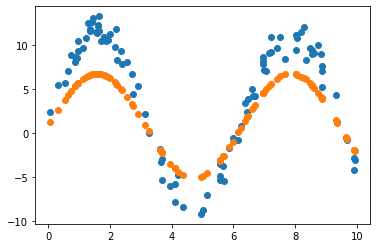
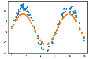
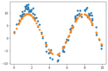
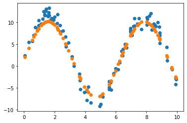
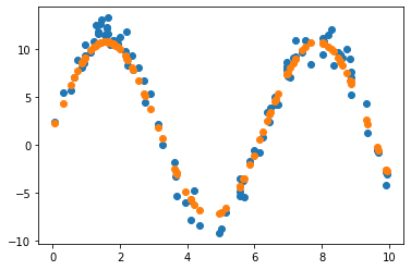
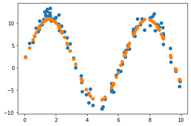
2.3.2 Learning rate = 0.01 조정

# Gradient Descent 구현 2
W = np.random.uniform(-1, 1)
b = np.random.uniform(-1, 1)

learning_rate = 0.01

for epoch in range(200):
  Y_Pred = W * np.sin(X) + b

  error = np.abs(Y_Pred - Y).mean()
  if error < 0.001:
    break

  # W, b의 Gradient 계산
  W_grad = learning_rate*((Y_Pred-Y)*X).mean()
  b_grad = learning_rate*((Y_Pred-Y)*1).mean()
  
  # W, b의 갱신
  W = W - W_grad
  b = b - b_grad

  if epoch % 20 == 0:
    Y_Pred = W * np.sin(X) + b
    plot_prediction(Y_Pred, Y)

output_19_0

output_19_1

output_19_2

output_19_3

output_19_4

output_19_5

output_19_6

output_19_7

output_19_8

output_19_9

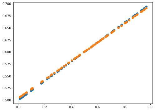
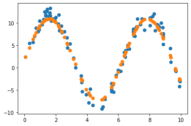
2.3.3 Learning rate = 0.01 & 노이즈 데이터로 원래 모델 파라미터 추정

# Gradient Descent 구현 3
W = np.random.uniform(-1, 1)
b = np.random.uniform(-1, 1)

learning_rate = 0.01

for epoch in range(200):
  Y_Pred = W * np.sin(X) + b

  error = np.abs(Y_Pred - Y_1).mean()
  if error < 0.001:
    break

  # W, b의 Gradient 계산
  W_grad = learning_rate*((Y_Pred-Y_1)*X).mean()
  b_grad = learning_rate*((Y_Pred-Y_1)*1).mean()
  
  # W, b의 갱신
  W = W - W_grad
  b = b - b_grad

  if epoch % 20 == 0:
    Y_Pred = W * np.sin(X) + b
    plot_prediction(Y_Pred, Y_1)

output_21_0

output_21_1

output_21_2

output_21_3

output_21_4

output_21_5

output_21_6

output_21_7

output_21_8

output_21_9

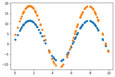
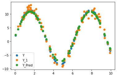
2.3.4 원래 값 vs 노이즈 포함 값 vs 예측 값

plt.scatter(X, Y, label = 'Y')
plt.scatter(X, Y_1, label = 'Y_1')
plt.scatter(X, Y_Pred, label = 'Y_Pred')
plt.legend(loc='lower left')
plt.show()

output_23_0

print(error)

0.9089337250354899

3. Discussion & Conclusion

Learning rate가 0.7인 경우, 직선 파라미터 추정은 잘 했으나 sine 함수 파라미터 추정은 잘 못하고 local minimum에 빠진듯 보입니다. 이후 Learning rate(LR)를 0.01로 수정하여 추정했을 때 sine 함수 파라미터를 잘 예측한 것으로 보아, 해당 문제에서 LR이 0.7은 굉장히 큰 폭으로 파라미터를 업데이트하는 것으로 생각됩니다. 지금의 예제에서는 결과를 보고 직접 LR을 조작하였으나, Adaptively or Automatically 최적의 LR을 도출할 수 있다면 좋을 것입니다.
2.3.4절의 그림을 보면, 원래 데이터에 노이즈를 포함시켜도 원래 모델에 대한 파라미터를 잘 추정할 수 있음을 확인할 수 있습니다.
사실 처음 실행의 결과가 잘 나왔지만, 사진 크기를 통일하려고 몇번이고 재실행했는데 원하는 결과가 나오지 않았습니다. 파라미터 초기치 설정에 대해서 재현성을 위한 코드를 추가하는 작업이 필요합니다.

4. References

Youtube 테디노트 TeddyNote, “경사하강법을 파이썬(python) 코드 구현”

Etc…

Gitblog 업로드를 위해서 “코랩 > 주피터노트북 > md 파일 다운로드 > 이미지 하나하나 첨부” 하는 고생을 했는데, 이미지 파일이 깨져서 보이지 않는 문제가 발생했습니다. 이거 해결하느라고 정말 개고생을 한거 같습니다… 해결하는 코드는 아래와 같습니다.
```

![output_7_0](../images/2022-07-24-techpost_2_GradientDescent/output_7_0.png)
   

<img src="/images/2022-07-24-techpost_2_GradientDescent/output_7_0.png" alt="output_7_0"> 
```
바꿨는데 문제는, 기존에는 그냥 드래그앤 드롭이었다면, 이제는 하나하나 복붙해서 일일이 값 수정해야 한다는 것입니다. ~~(아직 내가 멍청해서 노가다하는 걸지도 모르겠다…)~~
- 기존 Typora 드래그앤드롭 방법으로 이미지 업로드가 제대로 안 될 시 상기 방법을 사용하면 될 듯하고, 처음부터 수정된 코드를 활용하면 github repository 내에 이미지 업로드가 안되어 오류가 날 것으로 보입니다.
- 이러한 Gitblog 제작에 어려웠던 부분에 대해서는 따로 Category를 만들어 정리하도록 하겠습니다.
역시 많은 사람들에게 보여지는 것은 어려운 일입니다. 모든 블로거들 존경스럽습니다.
부족한 부분 코멘트해주세요 (:
Shout-out to J. Choi !

Twitter Facebook LinkedIn